Why VIX trackers don’t track the VIX, Part 2

In Part 1 of this post, we went over the details of the VIX and the ecosystem that surrounds it. We determined that VIX trackers like VXX lose money steadily in quiet markets because the VIX futures which make up their underlying portfolio are in contango. We now turn our attention to answering the question posed at the end of Part 1: why are VIX futures typically in contango? In the following sections, I will explore three possible explanations for this phenomenon.

The mean reversion explanation

The first way of explaining the contango present in the VIX is by reference to its historically mean-reverting behavior. The VIX is not a stake in a business with cash flows or a commodity with measurable supply and demand; it is a number which represents the level of uncertainty investors have about equities prices in the near future. We expect this number to change over time as macroeconomic conditions create more or less uncertainty. But there is a cyclicality to these changes, which gives the VIX a tendency towards mean reversion that is not present in regular assets.

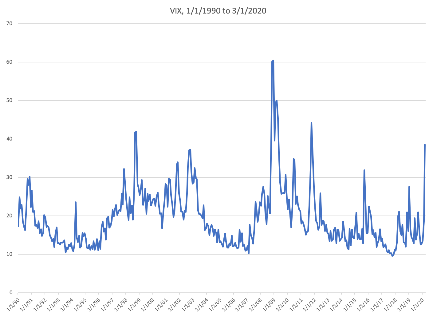
Here is a chart of monthly VIX values over the past thirty years. It has a few characteristics worth noting. For one thing, we can see that the VIX spends most of its time in a relatively narrow range. Arbitrarily choosing values of 12 and 24 as our floor and ceiling, we find that the VIX spends 70% of the thirty-year period within this band.

Furthermore, when the VIX does move away from its middle range, it typically doesn’t stay away for too long. The VIX’s average value over the thirty-year period is about 19. The longest period of time it spent strictly below this average was 20 months, and the longest period strictly above it was 16 months. So historically, whenever the VIX has moved away from its long-term average, it has always been relatively quick to return.

Of course, it’s always risky to assume the future will resemble the past. But if we generalize this behavior, we can build a simple mean-reverting model of future VIX values. According to this model, although the expected value of the VIX tomorrow is predominately a function of its value today, the expected value of the VIX a year from now is more heavily influenced by its historical average. The expected value of the VIX at some future point in time will converge towards the historical average as the time frame under consideration increases.

In a period when volatility is low relative to the historical average, as it was at the beginning of this year, our mean-reverting model expects the VIX to eventually bounce back up. Pricing VIX futures contracts based on this model would cause these contracts to be worth more as the time to expiration increases. And indeed, that is exactly the pattern we see when the futures are in contango. So if other traders are modeling the VIX as mean-reverting over the long term and trading its futures accordingly, that would explain the shape we see in the futures curve.

There is a corollary to this explanation for the VIX futures contango, which is that when the VIX is above its long-term historical average, we can expect it to eventually revert downward. This model of expected VIX values implies that the prices of VIX futures with longer times to expiration should be lower, shifting the futures curve into backwardation. And indeed that is exactly what we see in practice.

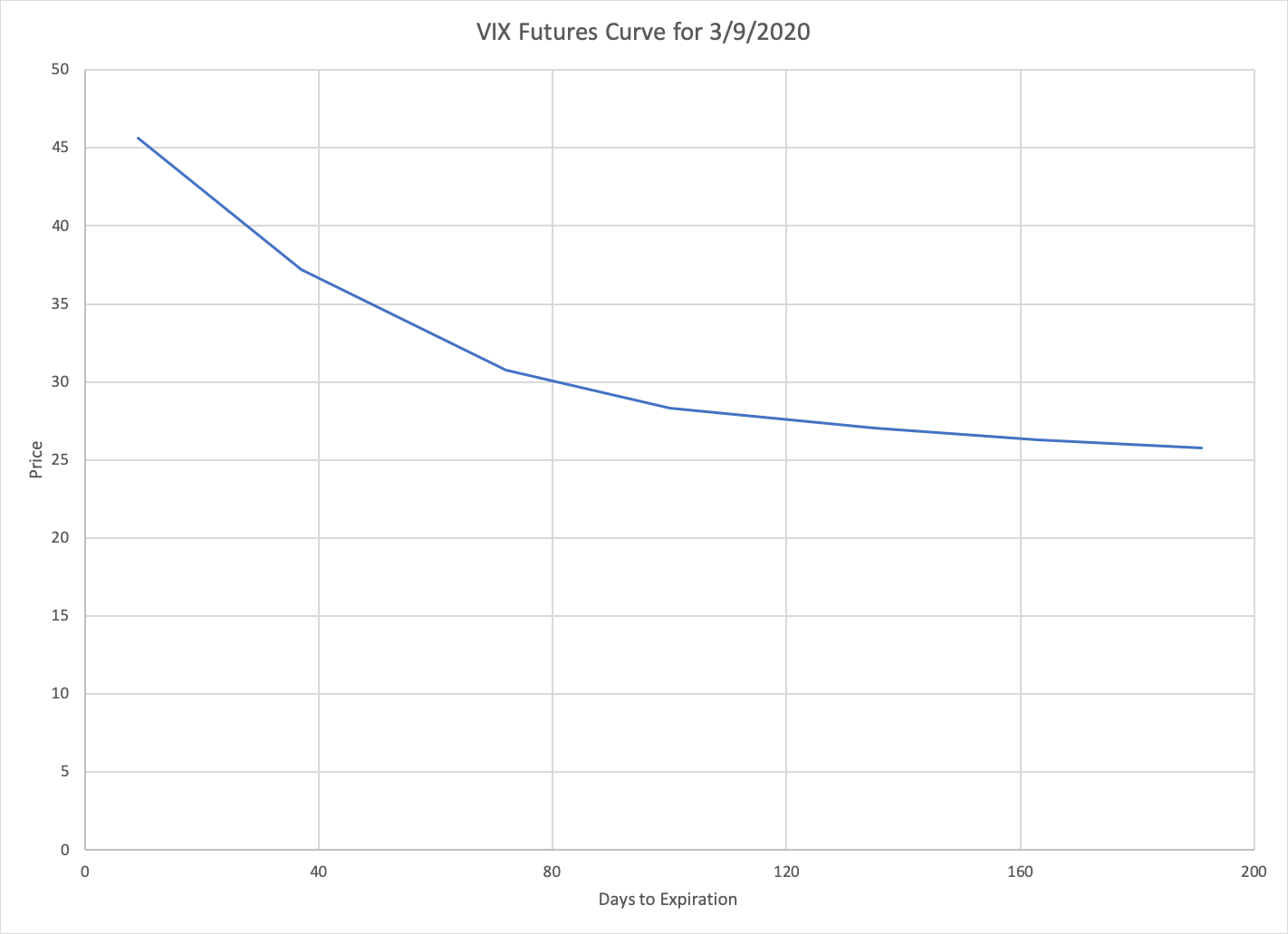
This chart shows the futures curve for the VIX at the end of the day on March 9, after the S&P fell so quickly that it tripped the NYSE’s circuit breakers for the first time in twenty years. The backwardation in this case is even sharper than the contango was back in January. This too is consistent with the historical behavior of the VIX — both because periods of abnormally high values tend to be shorter than periods of abnormally low values, and because the value of the VIX on March 9 was higher above the historical mean than the value on January 2 was below it.

Note that the backwardation of VIX futures when volatility is high means that inverse VIX trackers like SVXY (and the ill-fated XIV) will suffer the same problems during these periods as the regular trackers do under normal circumstances. That is, if the VIX has spiked and you buy SVXY as a way to bet on a reversion, the value of your position will quickly erode as long as the VIX remains elevated. This makes trading both long and short volatility products as much about timing as direction.

The options pricing explanation

A second explanation of the VIX futures contango comes from options prices. As noted earlier, while the value of the VIX represents the market’s estimate of near-term volatility, the way this estimate is actually calculated is based on options prices. This is possible because the non-linear payoff profile of options causes their prices to implicitly encode expectations about the volatility of the underlying asset. The VIX uses the prices of options expiring in 30 days to extract an estimate of the volatility over this period.

In light of this methodology, we can look to options prices for an alternate explanation of the shape of the VIX futures curve. Specifically, if it turns out that the prices of options with maturity dates further in the future imply a greater expectation of volatility, then the contango in VIX futures would be completely understandable. In that case, it isn’t so much that VIX futures become more expensive over time — it’s that expectations of volatility increase with time, and VIX futures prices increase accordingly.

One way to test this theory is to look at the term structure of implied volatility. That is, we could plot the implied volatility of S&P options as a function of their time to maturity. If implied volatility increases as a function of time to maturity, that would suggest that the fair price of VIX futures is indeed higher for later-dated contracts.

However, this approach isn’t quite right, because the measure of volatility represented by the VIX is distinct from the concept of implied volatility. Implied volatility derives an estimate of expected volatility using the price of a single option and a specific options pricing model, typically Black-Scholes. The VIX, on the other hand, is based on the full replication of a variance swap using a strip of options. As noted in the paper where the VIX formula is originally derived, the formula “provides a direct connection between the market cost of options and the strategy for capturing future realized volatility, even when there is an implied volatility skew and the simple Black-Scholes formula is invalid.”

In other words, an analysis based on (Black-Scholes) implied volatility is incomplete because it makes assumptions about the log-normality of asset prices which the VIX does not. A model-agnostic way to check whether VIX futures are fairly priced relative to their underlying options is to use the VIX formula itself. The value of the VIX at present is based on the weighted average price of options expiring 30 days from now. So we can construct an estimate for the value of the VIX at some date in the future by applying the same formula to the prices of options expiring 30 days after that date.

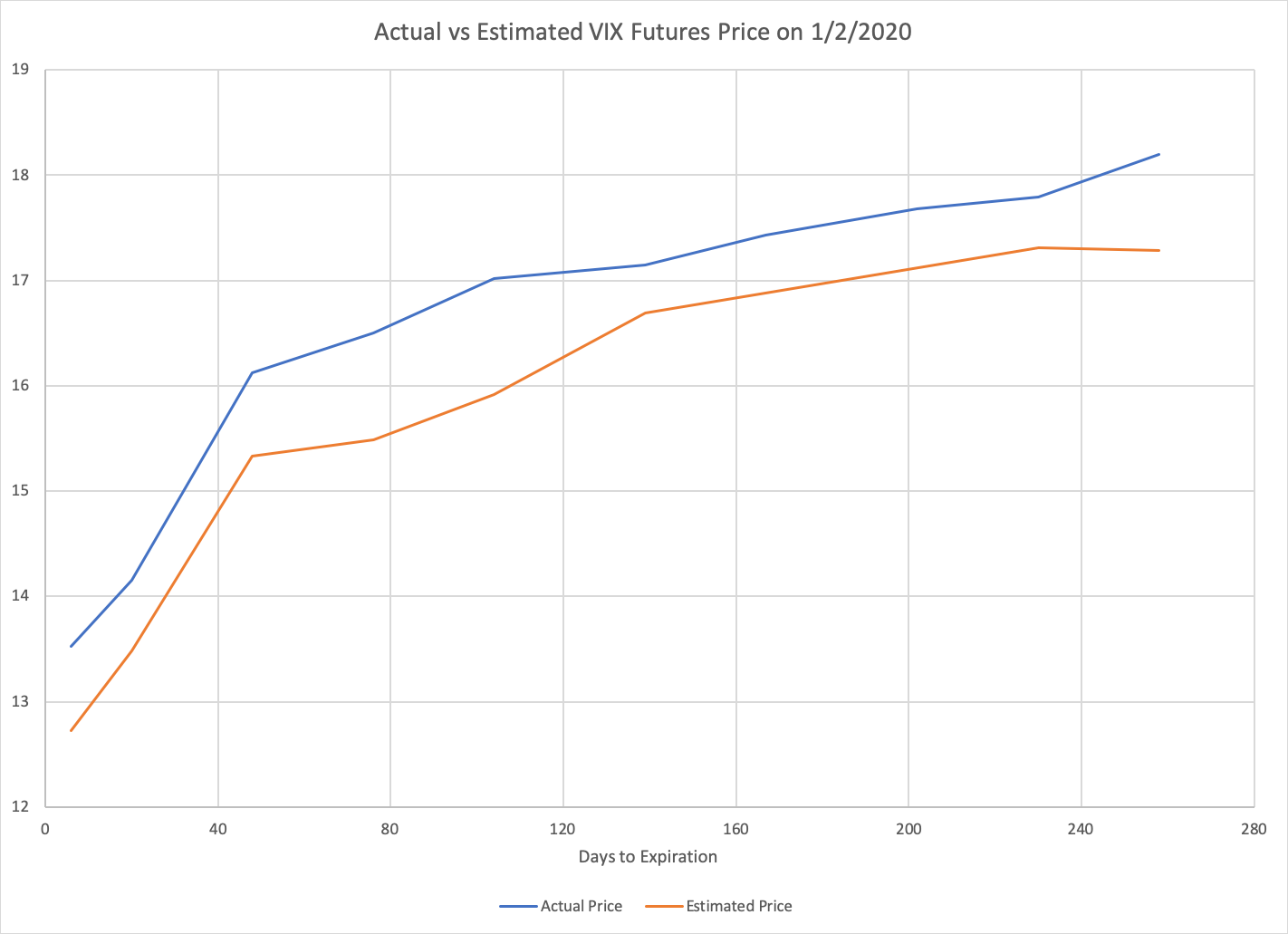
This chart shows the estimated values we get by applying the VIX formula to S&P options prices at the beginning of this year for various expiration dates. These values are plotted side-by-side with the actual prices of VIX futures expiring 30 days earlier. We can see that our options-based estimate of VIX futures values tracks very closely with the corresponding prices of VIX futures.

Note that our estimates of fair VIX future prices still aren’t completely right. We are using the prices of options expiring in four months (for example) to estimate the value of the VIX in three months. But the value of the VIX in three months represents an estimate of volatility during only month four, whereas the price of four-month options at present represents an estimate of volatility from now through month four. So what we’re really estimating is the value of an alternate version of the VIX which represents expected volatility over the next four months rather than the next thirty days.

To be completely accurate, we would need to also use the prices of three-month options to subtract out the expected volatility from now through month three, isolating the volatility expected during month four. However, this calculation is more involved and beyond the scope of this article. We will settle for noting that our current approach should be an underestimate — because the near-term expected volatility erroneously included is lower than the longer-term expected volatility — and that our estimate reassuringly tracks just below the actual VIX futures price. Our rough approach is sufficient to support the second explanation of VIX futures contango: options prices themselves imply an expectation of increasing volatility over time, and the contango in VIX futures is merely a reflection of this fact.

The efficient markets explanation

The final and most practical way to explain the contango in the VIX futures is to ask what would happen if they weren’t in contango. This explanation is a form of financial reductio ad absurdum.

Suppose that the price of a one-year VIX future was equal to the value of the VIX today. Or equivalently, suppose that the contracts expiring this month had the same price as those expiring next month, so you could roll your short-term position without a loss of value. In this case, continuously rolling a long position in VIX futures would be essentially the same as holding an asset whose price is equal to the VIX.

It turns out that having an asset with returns equal to the VIX is enormously useful from a portfolio construction perspective. Why? Because the VIX has two key properties.

First, there is a strong inverse correlation between the return of equities as a class and the value of the VIX. This is because volatility tends to be lower during bull markets and higher during bear markets. A more colorful way to say this is that markets “take the stairs up and the elevator down”. To put a number on it, the correlation between the monthly changes of SPX and VIX over the past 30 years is -0.65.

Second, note that the long-term expected “return” of the VIX is negligible. On January 2, 1990, the value of the VIX at market open was 17.24. Exactly thirty years later, the value of the VIX at market open was 13.46. That means if you “bought” the VIX thirty years ago and held it until now, your average annual loss would be less than 1%.

These two characteristics — negative correlation and near-zero expected return — make the VIX a natural hedge for anyone holding equities. We can demonstrate this by considering a portfolio with 80% allocated to tracking SPX and 20% allocated to VIX futures, rebalanced on a monthly basis. Compared to the vanilla portfolio invested 100% in an SPX tracker, this hedged portfolio has both higher annualized return (12% vs 7%) and lower standard deviation (12% vs 15%).

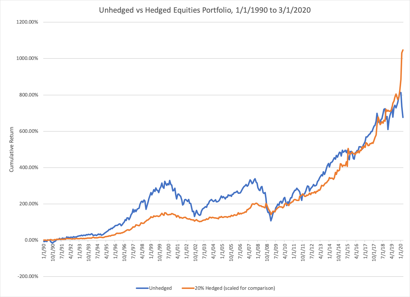
In other words, long exposure to the VIX provides a form of insurance which is strictly beneficial for a portfolio that is long equities. This fact makes everyone with a net long position in equities (so basically anyone with a retirement account) a natural buyer of this insurance. But of course, this demand will drive up the price of such insurance, until the price is commensurate with the benefit it provides.

Furthermore, the benefit of long exposure to the VIX is continuous in time: every additional month that you hold this insurance is a month where your overall portfolio looks better on a risk-adjusted basis. So we would expect buyers of this insurance to pay more for longer-lasting policies. And that is exactly what we see when VIX futures are in contango: a contract expiring in six months provides insurance for a longer period than a contract expiring in three, and so the six month contract also carries a higher premium.

In other words, if we lived in a world where it was possible to track the VIX perfectly via futures, then every savvy investor with an equities-heavy portfolio would be buying them. Ipso facto, VIX futures are more expensive in proportion to how much portfolio insurance they provide, and as a result cannot be used to track the underlying index for free.

Conclusion

In this post, we explored three different explanations for what causes a contango in VIX futures — the mean reversion explanation, the options pricing explanation, and the efficient markets explanation.

Note that all of these explanations are interrelated. One and two are connected because it is not the VIX specifically but volatility itself which is mean-reverting, and the market’s recognition of this fact causes options prices to imply higher levels of expected volatility further in the future. One and three are related because the mean-reverting nature of the VIX implies that it has near-zero expected return, which is a key component of the third explanation. And two and three are connected because we can also provide an efficient markets explanation for the increasing expectation of volatility over time implied by options prices — namely that buying puts is another form of portfolio-improving insurance.

In this sense, we can think of these explanations as three sides of the same coin. They represent different ways of characterizing the same underlying reality. If you can think of any other ways to interpret the contango of VIX futures, feel free to leave a comment, and thanks for reading!